Describing Places

Introduction

In this lab, we’ll learn some techniques for creating publication-quality summary tables while working to tell policy-relevant stories about places.

In addition to thinking about the basics of how we describe places, we will perform a basic policy analysis of the location of federal Opportunity Zones. This analysis will help illustrate how we can strategically build layers of stories. We’ll add some basic information about all census tracts so that we can describe the differences between ineligible, eligible but not designated, and eligible and designated census tracts.

Goals

Set up your computer so that RStudio can communicate with your Github account.

Core Concepts

This lab asks you to practice some basic data manipulation and management skills using the dplyr package.

Introduce several commonly used demographic indicators from the census
Introduce how to join datasets together based upon a common field
Introduce how to recode and classify data based upon one or more characteristics

Let’s get going…

Github Lab Repository

If you have not already done so, follow this link to accept the lab Github Classroom assignment repository.

Principles of Tidy Data

In the book R for Data Science, Hadley Wickam describes three principles for tidy data:

Each variable must have its own column
Each observation must have its own row
Each value must have its own cell

Much of the data we work with in the context of basic planning and policy analysis applications already conforms to this format (or is easily transformed into this format). This makes packages like tidyverse particularly useful for the common types of data manipulation that we perform.

While we’ll occasionally use base r coding over the course of the semester, for the most part, we’ll rely upon the tidyverse suite to help us. Let’s explore some basic command syntax.

Load Example Data

We’re going to work with a dataset that describes those census tracts that were designated as Opportunity Zones as part of the federal Tax Cuts and Jobs Act. These incentives are designed to spur investment in low-income and undercapitalized cities, by providing investors with tax incentives to invest capital in these locations.

The specific dataset which we’ll work with was developed by the Urban Institute, and adds to basic identification of designated census tracts some additional analysis of the characteristics of those places.

Loading Required Packages

We’re already learned how to use install.packages() and library() to (respectively) install and load packages that extend R and RStudio’s functionality. As a reminder, install.packages() downloads the package from a central server and installs it on your computer. You only have to install a package once. Using library() loads that package for use in your current RStudio session. If you plan to use that package in a given analysis, you’ll need to load it. To stay organized, you should load packages at the beginning of your script or markdown document.

Note that to install the package, you need to treat the package name as a character vector "tidyverse", but when you load it in your R session, it does not need to be treated as a character vector tidyverse because it is an object that R recognizes after it is installed.

We are going to load the following packages:

tidyverse contains tools which we’ll use to subset, filter, group, and summarize our data
readxl contains tools which will help us to read Excel files into R
gt contains tools for making nicely formatted tables.

Code

library(tidyverse)
library(readxl)
library(gt)

The read_xlsx() command from the readxl package will read Microsoft Excel files into data tables. Let’s start by loading the Urban Institute Opportunity Zone dataset:

Let’s read the Excel data and place it in an object called “ozs”:

Code

ozs <- read_xlsx("data/urbaninstitute_tractlevelozanalysis_update1242018.xlsx")

You can either do a Google search for Readxl to find documentation, or you can use R’s built in documentation by typing ?readxl

As the documentation states, readxl imports excel files. Looking at the documentation, the read_excel() command will read a single excel sheet, or we can optionally select a sheet by name or number from an excel workbook with multiple sheets. In this case, the Urban Institute data is in a workbook with a single sheet, so we just need to tell R where the file is to load.

Describing Data

One of the first steps that we should do when we load an unfamiliar dataset is to get to know it using some basic description commands.

Let’s use the str() command to analyze the dataset’s structure:

Code

str(ozs)

tibble [42,176 × 27] (S3: tbl_df/tbl/data.frame)
 $ geoid                : chr [1:42176] "01001020200" "01001020300" "01001020700" "01001020802" ...
 $ state                : chr [1:42176] "Alabama" "Alabama" "Alabama" "Alabama" ...
 $ Designated           : num [1:42176] NA NA 1 NA NA NA NA 1 NA 1 ...
 $ county               : chr [1:42176] "Autauga County" "Autauga County" "Autauga County" "Autauga County" ...
 $ Type                 : chr [1:42176] "Low-Income Community" "Non-LIC Contiguous" "Low-Income Community" "Non-LIC Contiguous" ...
 $ dec_score            : num [1:42176] 4 6 9 10 5 6 6 9 10 9 ...
 $ SE_Flag              : num [1:42176] NA NA NA NA NA NA NA NA NA NA ...
 $ Population           : num [1:42176] 2196 3136 3047 10743 2899 ...
 $ medhhincome2014_tract: num [1:42176] 41107 51250 45234 61242 49567 ...
 $ PovertyRate          : num [1:42176] 0.24 0.107 0.19 0.153 0.151 ...
 $ unemprate            : num [1:42176] 0.0775 0.051 0.1407 0.0459 0.0289 ...
 $ medvalue             : num [1:42176] 95300 113800 93500 160400 102900 ...
 $ medrent              : num [1:42176] 743 817 695 1018 546 ...
 $ pctown               : num [1:42176] 0.628 0.703 0.711 0.823 0.83 ...
 $ severerentburden     : num [1:42176] 0.3269 0.3223 0.3887 0.1994 0.0994 ...
 $ vacancyrate          : num [1:42176] 0.0584 0.1399 0.0619 0.0609 0.2182 ...
 $ pctwhitealone        : num [1:42176] 0.439 0.671 0.833 0.814 0.726 ...
 $ pctblackalone        : num [1:42176] 0.5187 0.205 0.0922 0.1572 0.2456 ...
 $ pctHispanic          : num [1:42176] 0.01275 0.0727 0.0338 0.01368 0.00448 ...
 $ pctAAPIalone         : num [1:42176] 0.01093 0.01052 0 0.00959 0 ...
 $ pctunder18           : num [1:42176] 0.218 0.224 0.249 0.27 0.245 ...
 $ pctover64            : num [1:42176] 0.124 0.175 0.149 0.122 0.156 ...
 $ HSorlower            : num [1:42176] 0.581 0.464 0.544 0.45 0.621 ...
 $ BAorhigher           : num [1:42176] 0.162 0.219 0.113 0.229 0.136 ...
 $ Metro                : num [1:42176] 1 1 1 1 1 1 1 1 1 1 ...
 $ Micro                : num [1:42176] NA NA NA NA NA NA NA NA NA NA ...
 $ NoCBSAType           : num [1:42176] NA NA NA NA NA NA NA NA NA NA ...

We get a list where each row is a variable in the dataset. We also learn more about the format of the variable (e.g. character, numeric), the number of observations, and we see examples of the first few observations.

Let’s next use summary() to get a statistical summary of each variable:

Code

summary(ozs)

    geoid              state             Designated       county         
 Length:42176       Length:42176       Min.   :1       Length:42176      
 Class :character   Class :character   1st Qu.:1       Class :character  
 Mode  :character   Mode  :character   Median :1       Mode  :character  
                                       Mean   :1                         
                                       3rd Qu.:1                         
                                       Max.   :1                         
                                       NA's   :33414                     
     Type             dec_score         SE_Flag        Population   
 Length:42176       Min.   : 1.000   Min.   :1       Min.   :    0  
 Class :character   1st Qu.: 3.000   1st Qu.:1       1st Qu.: 2752  
 Mode  :character   Median : 5.000   Median :1       Median : 3897  
                    Mean   : 5.495   Mean   :1       Mean   : 4147  
                    3rd Qu.: 8.000   3rd Qu.:1       3rd Qu.: 5224  
                    Max.   :10.000   Max.   :1       Max.   :40616  
                    NA's   :1253     NA's   :41111   NA's   :112    
 medhhincome2014_tract  PovertyRate       unemprate          medvalue      
 Min.   :  2499        Min.   :0.0000   Min.   :0.00000   Min.   :   9999  
 1st Qu.: 32014        1st Qu.:0.1380   1st Qu.:0.05900   1st Qu.:  85700  
 Median : 41094        Median :0.2055   Median :0.08734   Median : 122400  
 Mean   : 42153        Mean   :0.2331   Mean   :0.10063   Mean   : 165663  
 3rd Qu.: 50833        3rd Qu.:0.2996   3rd Qu.:0.12600   3rd Qu.: 191300  
 Max.   :181406        Max.   :1.0000   Max.   :1.00000   Max.   :2000001  
 NA's   :249           NA's   :141      NA's   :141       NA's   :1106     
    medrent           pctown       severerentburden  vacancyrate     
 Min.   :  99.0   Min.   :0.0000   Min.   :0.0000   Min.   :0.00000  
 1st Qu.: 655.0   1st Qu.:0.3833   1st Qu.:0.1662   1st Qu.:0.07115  
 Median : 800.0   Median :0.5728   Median :0.2403   Median :0.11658  
 Mean   : 860.9   Mean   :0.5436   Mean   :0.2476   Mean   :0.14120  
 3rd Qu.:1010.0   3rd Qu.:0.7316   3rd Qu.:0.3206   3rd Qu.:0.18011  
 Max.   :3501.0   Max.   :1.0000   Max.   :1.0000   Max.   :1.00000  
 NA's   :395      NA's   :1033     NA's   :189      NA's   :167      
 pctwhitealone    pctblackalone      pctHispanic       pctAAPIalone    
 Min.   :0.0000   Min.   :0.00000   Min.   :0.00000   Min.   :0.00000  
 1st Qu.:0.2040   1st Qu.:0.01072   1st Qu.:0.02602   1st Qu.:0.00000  
 Median :0.5614   Median :0.06656   Median :0.09304   Median :0.00883  
 Mean   :0.5211   Mean   :0.18652   Mean   :0.22060   Mean   :0.03806  
 3rd Qu.:0.8294   3rd Qu.:0.25000   3rd Qu.:0.32014   3rd Qu.:0.03533  
 Max.   :1.0000   Max.   :1.00000   Max.   :1.00000   Max.   :0.91144  
 NA's   :131      NA's   :131       NA's   :131       NA's   :131      
   pctunder18       pctover64         HSorlower        BAorhigher    
 Min.   :0.0000   Min.   :0.00000   Min.   :0.0000   Min.   :0.0000  
 1st Qu.:0.1908   1st Qu.:0.09436   1st Qu.:0.4150   1st Qu.:0.1120  
 Median :0.2300   Median :0.13604   Median :0.5182   Median :0.1679  
 Mean   :0.2295   Mean   :0.14340   Mean   :0.5067   Mean   :0.2034  
 3rd Qu.:0.2719   3rd Qu.:0.18057   3rd Qu.:0.6113   3rd Qu.:0.2536  
 Max.   :0.6468   Max.   :1.00000   Max.   :1.0000   Max.   :1.0000  
 NA's   :131      NA's   :131       NA's   :132      NA's   :132     
     Metro          Micro         NoCBSAType   
 Min.   :1      Min.   :1       Min.   :1      
 1st Qu.:1      1st Qu.:1       1st Qu.:1      
 Median :1      Median :1       Median :1      
 Mean   :1      Mean   :1       Mean   :1      
 3rd Qu.:1      3rd Qu.:1       3rd Qu.:1      
 Max.   :1      Max.   :1       Max.   :1      
 NA's   :9111   NA's   :37448   NA's   :37793

This gives us a statistical summary including distribution and central tendency statistics, as well as information on the number of values that are NA.

A few things to note after your preliminary inspection:

These data are at the census tract level and include geographic identifiers including geoid, the combined, state-county-tract FIPS code, state the state name, and county the county name.
These data include a field named Designated which is 1 when an eligible tract was designated as an opportunity zone, and NA where the tract was not designated.
The dataset also includes some other tract-level demographic measures, as well as additional geographic flags (variables that take the value 0 or 1).

Query and Describe the Data

The dataset we’re looking at is for the entire United States. We can easily summarize characteristics of the entire dataset.

Recoding Values

One of the characteristics tracked in the Urban Institute data is the median household income for each designated census tract. We might question whether there’s a difference in the median household income for designated and not-designated but eligible census tracts. This may help us understand something about whether the most needy tracts were selected from those that are eligible.

How would we do this? Conceptually…

We need to split our data into designated and not designated census tracts, and then calculate the average of the median income separately for these tracts.
Before we do this, let’s take care of one bit of housekeeping. The Urban Institute has coded the designated variable as either taking a value of 1 when designated or NA when not. Let’s recode those NA values to equal 0 instead.
To recode, we need to select those values from the Designated column in the ozs data frame where the value is NA and overwrite them with a new value of 0.

There’s lots of ways we could do this:

Strategy 1 - Conditional Statement

We could use a conditional statement ifelse() to specify that if a value is NA in the Designated column we change it to 0.

Code

ozs |> 
  mutate(Designated = ifelse(is.na(Designated), 0, Designated))

# A tibble: 42,176 × 27
   geoid       state   Designated county      Type  dec_score SE_Flag Population
   <chr>       <chr>        <dbl> <chr>       <chr>     <dbl>   <dbl>      <dbl>
 1 01001020200 Alabama          0 Autauga Co… Low-…         4      NA       2196
 2 01001020300 Alabama          0 Autauga Co… Non-…         6      NA       3136
 3 01001020700 Alabama          1 Autauga Co… Low-…         9      NA       3047
 4 01001020802 Alabama          0 Autauga Co… Non-…        10      NA      10743
 5 01001021000 Alabama          0 Autauga Co… Non-…         5      NA       2899
 6 01001021100 Alabama          0 Autauga Co… Low-…         6      NA       3247
 7 01003010100 Alabama          0 Baldwin Co… Non-…         6      NA       4013
 8 01003010200 Alabama          1 Baldwin Co… Low-…         9      NA       3067
 9 01003010300 Alabama          0 Baldwin Co… Non-…        10      NA       8079
10 01003010400 Alabama          1 Baldwin Co… Non-…         9      NA       4578
# ℹ 42,166 more rows
# ℹ 19 more variables: medhhincome2014_tract <dbl>, PovertyRate <dbl>,
#   unemprate <dbl>, medvalue <dbl>, medrent <dbl>, pctown <dbl>,
#   severerentburden <dbl>, vacancyrate <dbl>, pctwhitealone <dbl>,
#   pctblackalone <dbl>, pctHispanic <dbl>, pctAAPIalone <dbl>,
#   pctunder18 <dbl>, pctover64 <dbl>, HSorlower <dbl>, BAorhigher <dbl>,
#   Metro <dbl>, Micro <dbl>, NoCBSAType <dbl>

In dplyr syntax, what we said here was with reference to the ozs dataset ozs |> let’s alter the dataset mutate(). Let’s alter the column named Designated mutate(Designated = ). Let’s alter the column named Designated conditionally mutate(Designated = ifelse()). If the value of Designated is equal to NA, replace it with 0, otherwise keep the value present in the Designated observation mutate(Designated = ifelse(is.na(Designated), 0, Designated)).

Looking at this ifelse() statement, you might have been tempted to write something like Designated ==NA`which will not work.is.na()is the proper logical test to return whether a value is or is notNA`.

Strategy 2: Use a Specialized Command

We could use a specialized command such as replace_na() from the tidyr package to replace our NA values:

Code

ozs |> 
  mutate(Designated = replace_na(Designated, 0))

# A tibble: 42,176 × 27
   geoid       state   Designated county      Type  dec_score SE_Flag Population
   <chr>       <chr>        <dbl> <chr>       <chr>     <dbl>   <dbl>      <dbl>
 1 01001020200 Alabama          0 Autauga Co… Low-…         4      NA       2196
 2 01001020300 Alabama          0 Autauga Co… Non-…         6      NA       3136
 3 01001020700 Alabama          1 Autauga Co… Low-…         9      NA       3047
 4 01001020802 Alabama          0 Autauga Co… Non-…        10      NA      10743
 5 01001021000 Alabama          0 Autauga Co… Non-…         5      NA       2899
 6 01001021100 Alabama          0 Autauga Co… Low-…         6      NA       3247
 7 01003010100 Alabama          0 Baldwin Co… Non-…         6      NA       4013
 8 01003010200 Alabama          1 Baldwin Co… Low-…         9      NA       3067
 9 01003010300 Alabama          0 Baldwin Co… Non-…        10      NA       8079
10 01003010400 Alabama          1 Baldwin Co… Non-…         9      NA       4578
# ℹ 42,166 more rows
# ℹ 19 more variables: medhhincome2014_tract <dbl>, PovertyRate <dbl>,
#   unemprate <dbl>, medvalue <dbl>, medrent <dbl>, pctown <dbl>,
#   severerentburden <dbl>, vacancyrate <dbl>, pctwhitealone <dbl>,
#   pctblackalone <dbl>, pctHispanic <dbl>, pctAAPIalone <dbl>,
#   pctunder18 <dbl>, pctover64 <dbl>, HSorlower <dbl>, BAorhigher <dbl>,
#   Metro <dbl>, Micro <dbl>, NoCBSAType <dbl>

Note that in replace_na() we are specifying the column we want to replace the NA value in as well as the value we want to replace NA with.

Strategy 3: Recode and Change Format

Depending upon what we wanted to do with our Designated labels, we could simultaneously deal with recoding our NA values and relabeling the values for legibility. case_when() is useful for these more complex operations:

Code

ozs |> mutate(
  Designated = case_when(
    Designated == 1 ~"Designated",
    is.na(Designated) ~"Not Designated"
))

# A tibble: 42,176 × 27
   geoid       state   Designated     county  Type  dec_score SE_Flag Population
   <chr>       <chr>   <chr>          <chr>   <chr>     <dbl>   <dbl>      <dbl>
 1 01001020200 Alabama Not Designated Autaug… Low-…         4      NA       2196
 2 01001020300 Alabama Not Designated Autaug… Non-…         6      NA       3136
 3 01001020700 Alabama Designated     Autaug… Low-…         9      NA       3047
 4 01001020802 Alabama Not Designated Autaug… Non-…        10      NA      10743
 5 01001021000 Alabama Not Designated Autaug… Non-…         5      NA       2899
 6 01001021100 Alabama Not Designated Autaug… Low-…         6      NA       3247
 7 01003010100 Alabama Not Designated Baldwi… Non-…         6      NA       4013
 8 01003010200 Alabama Designated     Baldwi… Low-…         9      NA       3067
 9 01003010300 Alabama Not Designated Baldwi… Non-…        10      NA       8079
10 01003010400 Alabama Designated     Baldwi… Non-…         9      NA       4578
# ℹ 42,166 more rows
# ℹ 19 more variables: medhhincome2014_tract <dbl>, PovertyRate <dbl>,
#   unemprate <dbl>, medvalue <dbl>, medrent <dbl>, pctown <dbl>,
#   severerentburden <dbl>, vacancyrate <dbl>, pctwhitealone <dbl>,
#   pctblackalone <dbl>, pctHispanic <dbl>, pctAAPIalone <dbl>,
#   pctunder18 <dbl>, pctover64 <dbl>, HSorlower <dbl>, BAorhigher <dbl>,
#   Metro <dbl>, Micro <dbl>, NoCBSAType <dbl>

What’s going on here? case_when() allows us to conditionally recode values. We specify the condition and then what to do when that condition is met. For instance, we specify the condition Designated == 1 and then say when this condition is met, we want you to change that observation to Designated ~"Designated". We then say what to do if the value is NA - label it as “Not Designated”.

For the sake of legibility, let’s use the third strategy on our dataset:

Code

ozs <- ozs |> mutate(
  Designated = case_when(
    Designated == 1 ~"Designated",
    is.na(Designated) ~"Not Designated"
))

And here’s what our Designated column now looks like:

geoid	state	county	Designated
01001020200	Alabama	Autauga County	Not Designated
01001020300	Alabama	Autauga County	Not Designated
01001020700	Alabama	Autauga County	Designated
01001020802	Alabama	Autauga County	Not Designated
01001021000	Alabama	Autauga County	Not Designated
01001021100	Alabama	Autauga County	Not Designated

Summarizing Data

Now that we’ve recoded our designated column, let’s do some description of the characteristics of designated and not designated places.

Let’s use a combination of group_by() and summarise() to produce a summary table showing the mean value for designated and not designated census tracts.

Code

ozs |> 
  group_by(Designated) |> 
  summarise(Income = mean(medhhincome2014_tract))

# A tibble: 2 × 2
  Designated     Income
  <chr>           <dbl>
1 Designated         NA
2 Not Designated     NA

We getting a table back, but why did we get NA insted of numbers here? If you’ve ever used the average mean() command in R, you probably understand what’s going on here. As a safety measure, when you average values, R will return NA if any value in that series is NA. If you’re not expecting any NA values, this is good, becuase you’ll quickly discover that there are unexpected NA values in your dataset. We might expect a few census tracts with missing income values coded as NA, so we will want to indicate na.rm = TRUE here so that R removes those NAs when calculating the mean.

Code

ozs |> 
  group_by(Designated) |> 
  summarise(Income = mean(medhhincome2014_tract, na.rm=TRUE))

# A tibble: 2 × 2
  Designated     Income
  <chr>           <dbl>
1 Designated     33345.
2 Not Designated 44446.

Much better. We can see that that on average, the median household income for eligible designated census tracts is lower than that for eligible not designated census tracts. Since the Opportunity Zone legislation is designed to target distressed neighborhoods, this is a good sign that program targeting is focused on neighborhoods with greater need.

We might want to add some additional information to our summary table. One useful piece of information would be the number of census tracts that are designated or not designated.

Code

ozs |> 
  group_by(Designated) |> 
  summarise(
    Tracts = n(),
    Income = mean(medhhincome2014_tract, na.rm=TRUE))

# A tibble: 2 × 3
  Designated     Tracts Income
  <chr>           <int>  <dbl>
1 Designated       8762 33345.
2 Not Designated  33414 44446.

Within a summarise() statement, n() gives us a count of observations (rows) for each grouping. In this case, there are 8,762 census tracts designated as opportunity zones, and an additional 33,414 that were eligible based upon program criteria but not designated.

We could easily add other summaries to our summary table for this dataset, or further modify.

Filtering Data

Now that we have some sense for how we might produce basic summaries of our data, how can we query out (filter) observations by row? How, for instance, would you modify the above code to produce the same table for counties in Illinois?

We can use a filter() statement to easily accomplish this. filter() allows us to specify one (or more) criteria for which we want to select rows from a larger dataset.

Let’s take a step back and filter our base dataset to focus on observations in Illinois.

Code

ozs |> 
  filter(state == "Illinois")

# A tibble: 1,659 × 27
   geoid       state    Designated     county Type  dec_score SE_Flag Population
   <chr>       <chr>    <chr>          <chr>  <chr>     <dbl>   <dbl>      <dbl>
 1 17001000201 Illinois Not Designated Adams… Non-…         7      NA       1937
 2 17001000202 Illinois Not Designated Adams… Low-…         1      NA       2563
 3 17001000400 Illinois Not Designated Adams… Low-…         1      NA       3403
 4 17001000500 Illinois Not Designated Adams… Low-…         1      NA       2298
 5 17001000700 Illinois Not Designated Adams… Low-…         1      NA       1259
 6 17001000800 Illinois Designated     Adams… Low-…         1      NA       2700
 7 17001000900 Illinois Not Designated Adams… Low-…         5      NA       2671
 8 17001010100 Illinois Not Designated Adams… Non-…         2      NA       4323
 9 17001010200 Illinois Not Designated Adams… Low-…         2      NA       3436
10 17001010300 Illinois Not Designated Adams… Non-…         8      NA       6038
# ℹ 1,649 more rows
# ℹ 19 more variables: medhhincome2014_tract <dbl>, PovertyRate <dbl>,
#   unemprate <dbl>, medvalue <dbl>, medrent <dbl>, pctown <dbl>,
#   severerentburden <dbl>, vacancyrate <dbl>, pctwhitealone <dbl>,
#   pctblackalone <dbl>, pctHispanic <dbl>, pctAAPIalone <dbl>,
#   pctunder18 <dbl>, pctover64 <dbl>, HSorlower <dbl>, BAorhigher <dbl>,
#   Metro <dbl>, Micro <dbl>, NoCBSAType <dbl>

Recall that the ozs dataset has 42,176 observations (rows). We filtered the data using the criteria that the value of state is equal to “Illinois”, resulting in 1,659 observations (eligible census tracts in Illinois).

From here, we can re-use our prior code to produce a summary table that is focused on Illinois.

Code

ozs |> 
  filter(state == "Illinois") |> 
  group_by(Designated) |> 
  summarise(
    Tracts = n(),
    Income = mean(medhhincome2014_tract, na.rm=TRUE))

# A tibble: 2 × 3
  Designated     Tracts Income
  <chr>           <int>  <dbl>
1 Designated        327 30504.
2 Not Designated   1332 45281.

Ok - but how do we summarise by county? We just need to add that as an additional grouping criteria in our group_by() statement:

Code

ozs |> 
  filter(state == "Illinois") |> 
  group_by(county, Designated) |> 
  summarise(
    Tracts = n(),
    Income = mean(medhhincome2014_tract, na.rm=TRUE))

# A tibble: 181 × 4
# Groups:   county [95]
   county           Designated     Tracts Income
   <chr>            <chr>           <int>  <dbl>
 1 Adams County     Designated          1 26012 
 2 Adams County     Not Designated      9 39614.
 3 Alexander County Designated          1 21500 
 4 Alexander County Not Designated      3 32809 
 5 Bond County      Designated          1 49590 
 6 Bond County      Not Designated      1 52310 
 7 Boone County     Designated          1 40599 
 8 Boone County     Not Designated      2 45742 
 9 Bureau County    Designated          1 48083 
10 Bureau County    Not Designated      3 60339.
# ℹ 171 more rows

We are basically saying, group by both county and designated and then summarize for each.

With a few lines of code, we can produce very powerful and specific kinds of summaries for our data.

Pivoting Data

Our summary is getting more nuanced. We’ve used group_by() and summarise() to sumamrise data based upon certain characteristics. We’ve summarized in such a way where for our Illinois counties, we have two observations for each county - one that summarises values for designated tracts in that county, and one that summarises values for not designated tracts.

It might be useful for us to reshape our summary table so that there is one row for each county, with each row containing the summary value for both designated and not designated tracts.

The two commands pivot_wider() and pivot_longer() are useful for reshaping our data. pivot_wider() essentially adds columns to a dataset by transitioning content from rows to columns. pivot_longer() does the opposite - it makes a dataset longer by transitioning columns to rows.

In our case, let’s use pivot_wider() to transition our Designated and Not Designated rows into columns.

Code

ozs |> 
  filter(state == "Illinois") |> 
  group_by(county, Designated) |> 
  summarise(
    Tracts = n(),
    Income = mean(medhhincome2014_tract, na.rm=TRUE)) |> pivot_wider(names_from = Designated, values_from = Income)

# A tibble: 172 × 4
# Groups:   county [95]
   county           Tracts Designated `Not Designated`
   <chr>             <int>      <dbl>            <dbl>
 1 Adams County          1      26012              NA 
 2 Adams County          9         NA           39614.
 3 Alexander County      1      21500              NA 
 4 Alexander County      3         NA           32809 
 5 Bond County           1      49590           52310 
 6 Boone County          1      40599              NA 
 7 Boone County          2         NA           45742 
 8 Bureau County         1      48083              NA 
 9 Bureau County         3         NA           60339.
10 Calhoun County        2         NA           55290 
# ℹ 162 more rows

We start with our previous summary and pass two arguments to pivot_wider().

We use names_from to specify the column in our dataset contining row values that we want to become new columns. In this case we’d expect that our Desginated column would result in the creation of two new columns - one where values are Designated and one where values are Not Designated.

We use values_from to specify the column containing the values we want in our new columns, in this case, the average of tract income.

One problem though - our tract count column is still present and these values are not reshaped. To simplify things, let’s just get rid of this count so we can see what things look like:

Code

ozs |> 
  filter(state == "Illinois") |> 
  group_by(county, Designated) |> 
  summarise(
    Income = mean(medhhincome2014_tract, na.rm=TRUE)) |> pivot_wider(names_from = Designated, values_from = Income)

# A tibble: 95 × 3
# Groups:   county [95]
   county           Designated `Not Designated`
   <chr>                 <dbl>            <dbl>
 1 Adams County         26012            39614.
 2 Alexander County     21500            32809 
 3 Bond County          49590            52310 
 4 Boone County         40599            45742 
 5 Bureau County        48083            60339.
 6 Calhoun County          NA            55290 
 7 Carroll County       35184            58942 
 8 Cass County          37679            46840.
 9 Champaign County     13989.           45604.
10 Christian County     36164            45945.
# ℹ 85 more rows

Looking good! To make things a bit more informative, let’s also show the difference in income between designated and not designated tracts:

Code

ozs |> 
  filter(state == "Illinois") |> 
  group_by(county, Designated) |> 
  summarise(
    Income = mean(medhhincome2014_tract, na.rm=TRUE)) |> pivot_wider(names_from = Designated, values_from = Income) |> 
  mutate(Difference = Designated - `Not Designated`)

# A tibble: 95 × 4
# Groups:   county [95]
   county           Designated `Not Designated` Difference
   <chr>                 <dbl>            <dbl>      <dbl>
 1 Adams County         26012            39614.    -13602.
 2 Alexander County     21500            32809     -11309 
 3 Bond County          49590            52310      -2720 
 4 Boone County         40599            45742      -5143 
 5 Bureau County        48083            60339.    -12256.
 6 Calhoun County          NA            55290         NA 
 7 Carroll County       35184            58942     -23758 
 8 Cass County          37679            46840.     -9162.
 9 Champaign County     13989.           45604.    -31615.
10 Christian County     36164            45945.     -9781.
# ℹ 85 more rows

One note here - in the last mutate() statement, you see that Not Designated has backticks around it. This is because there’s a space between “Not” and “Designated” which will be treated as separate variable names. The backticks allow this to be referenced as a column. We could change the name to something like Not_Designated, but backticks will allow us to appropriately reference it as well.

Joining Tables

Linking together the place data to the ozs data might would give us some additional context regarding opportunity zones. Remember that the opportunity zones data itemizes those census tracts that were eligible for designation with the Designated column denoting which eligible census tracts actually became opportunity zones. If we link together information for census tracts which were not eligible for designation, we could learn something about the differences between undesignated, eligible not designated, and eligible designated census tracts.

In order to link together these two datasets, we need to learn about and apply relational joins to bring these two datasets together.

Joins Overview

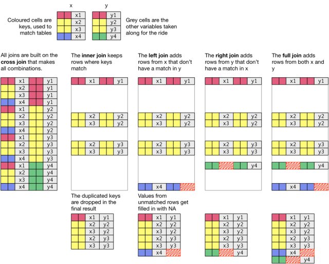
Joins are methods to merge two datasets based on common attributes. It’s rare that one single dataset contains all of the information you wish to tell a story about, so it’s important to understand how joins work.

A Venn diagram of join types.

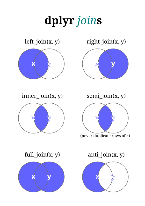The tidyverse package which we’ve installed and loaded in the past can perform seven different types of relational joins. We’ll discuss six of them briefly, but focus on four key types. Joins require us to have two tables with some type of common identifier column present in both that we can match records based on.

Join Types

Let’s assume we have two data frames named x and y, and we’re trying to match a column called key in both datasets.

left_join(): A left join returns every row in x and all the columns from x and y. If a value in the key column in x doesn’t exist in y, the row will contain NA values for all the y columns. If there are multiple key matches, all the possible combinations will be returned.
right_join(): This is similar to a left join, but returns every row in y instead.
inner_join(): An inner join returns all the rows in x where there is an key match in y, and all the columns in x and y.
full_join(): A full join returns all rows and all columns from x and y. If there isn’t a match in the x key column, all x columns will return NA. (The same is true for y.)
semi_join(): A semi-join returns the rows in x where there is an key match in y. It is different than an inner join in that it only returns the columns in x and doesn’t duplicate rows if there are multiple matches in y.
anti_join(): An anti-join returns the rows in x where there is not a matching key in y. It only returns the columns in x.

You’ll notice that only the first four joins—left, right, inner, and full—merge two datasets. Those are going to be the most valuable ones to learn. Here are a couple of additional illustrations to illustrate how joins work.

Join example 1 Join example 2 The basic general syntax for the joins is the same:

*_join(x, y, by = "key name")

x and y are self-explanatory. The by attribute is used to name the key, or the variable that the two datasets have in common. If you’re lucky, they’ll have the same name. If you’re unlucky, you’ll have to type a bit more: by = c("name1" = "name2"), assuming “name1” is the name of the key column in x and “name2” is the name of the key column in y.

Example

Let’s assume we have two data frames: fruit_1 that contains some characteristics about fruit, and fruit_2 that has some others. Here’s how they’re defined:

Note that the code above is just another syntax for creating tables as we did in the past.

Code

print(fruit_1)

# A tibble: 4 × 2
  fruit  color 
  <chr>  <chr> 
1 apple  red   
2 orange orange
3 banana yellow
4 lime   green

Code

print(fruit_2)

# A tibble: 4 × 3
  fruit  shape price
  <chr>  <chr> <dbl>
1 orange round  0.4 
2 banana long   0.3 
3 lime   oval   0.25
4 durian spiky  8

What would be the result of a left join, right join, and inner join of fruit_1 and fruit 2?

Note the following:

The left join includes all records from fruit_1, but excludes those measures from fruit_2 where there isn’t a match in the fruit column (durian). Note that even though there’s not shape and price information for apples in fruit_2, the rows are still included, but with NA where the data would be were it present.
The right join includes all records from fruit_2 but excludes those columns from fruit_1 where there isn’t a match in the fruit column. In this case, we’re missing color information for durian fruit.
The inner join includes only those records from fruit_1 and fruit_2 where there were matches in both datasets.

The powerful thing about these joins is that they allow us to bring together data with different shapes and we can control which elements of the data are joined. Joins will become far more intuitive as you use them more.

Joining Together OZs and Place datasets

Now that we have a sense for how joins work, let’s combine our oz and place into one larger table.

Code

place <- read_csv("data/place_name.csv")

Rows: 73057 Columns: 5
── Column specification ────────────────────────────────────────────────────────
Delimiter: ","
chr (5): STATEFP, COUNTYFP, TRACTCE, GEOID, place_name

ℹ Use `spec()` to retrieve the full column specification for this data.
ℹ Specify the column types or set `show_col_types = FALSE` to quiet this message.

Code

place

# A tibble: 73,057 × 5
   STATEFP COUNTYFP TRACTCE GEOID       place_name
   <chr>   <chr>    <chr>   <chr>       <chr>     
 1 01      001      020100  01001020100 Prattville
 2 01      001      020200  01001020200 Prattville
 3 01      001      020300  01001020300 Prattville
 4 01      001      020400  01001020400 Prattville
 5 01      001      020500  01001020500 Prattville
 6 01      001      020600  01001020600 Prattville
 7 01      001      020700  01001020700 Prattville
 8 01      001      020801  01001020801 <NA>      
 9 01      001      020802  01001020802 <NA>      
10 01      001      020900  01001020900 <NA>      
# ℹ 73,047 more rows

If you take a look at both tables, you’ll note that they have a field in common called geoid. This represents a unique code that is assigned to each census tract geography. Technically, this is a FIPS (Federal Information Processing Standards) code. FIPS codes for tracts are hierarchical - the first two digits are unique to each state, the next three digits correspond to each county, and the remaining six digits are unique to each census tract in that county.

Because each tract is labelled with corresponding FIPS codes, we can join the two datasets together based upon this common field. This will become a fairly common action for you that you will repeat over the course of this class.

Next, we should think carefully about what kind of join we want. We know we have ozs data for a subset of census tracts in the U.S. and we have the place data for a more expansive set of tracts. If we want to preserve the more extensive data (including those rows that do not match up with oz- eligible tracts), what type of join should we use and how would we construct it?

Just to make sure we get this correct, I’m going to provide you with the way to complete your first join on real data. We have one more issue to deal with here to successfully join our data together. Recall that join takes three arguments - two table objects to join together and at least one common field to complete the join based on. These columns are both labelled geoid, but one is capitalized and one is not. We’ll need to tell our join function that these two columns with different names (different in that one is capitalized and one is not) should be joined to each other. We use the modified by=c("GEOID" = "geoid") to denote that GEOID in the place data should be joined to geoid in the ozs data. If the names were the same (say, both were GEOID), we could simply say by="GEOID" and this would work.

Okay, with that out of the way, let’s join our data together:

Code

dataset<-left_join(place, ozs, by=c("GEOID" = "geoid"))

Into a new object called dataset, we joined all rows from place and those records from ozs that matched. Records from place without a match in ozs will have NA where there could be data.

Take a look at the data:

Code

View(dataset)

Start by looking at the number of rows in the data - 73,057 - the same number as in the place data - we have brought in all rows from the place data and have joined to in matching rows in the ozs data. It would be useful for us to start off by knowing how many rows fall into each of our three categories - ineligible for designated, eligible and undesignated, and eligible and designated. At this point, the NA values in the Designated column reflect ineligible, the 0’s in that column reflect eligible but not designated, and the 1’s represent eligible and designated.

Use your new knowledge of dplyr’s group_by() and summarise() to create a summary table based upon the three values that we expect the Designated column to take. You’ve learned that you could define what type of summary you’d like to produce in your summarise() statement. Let’s use n() which counts the number of rows that meet each category specified in group_by():

Code

dataset |> 
  group_by(Designated) |> 
  summarise(n())

# A tibble: 3 × 2
  Designated     `n()`
  <chr>          <int>
1 Designated      7825
2 Not Designated 33391
3 <NA>           31841

You should see that we have 31,841 rows (census tracts) that were ineligible for designation, an additional 33,391 that were eligible but not designated, and 7,825 that were eligible and designated. Excellent!

What might you want to do next to be able to properly label the three categories that now exist for designated?

Making Nice Tables

As many of you have remarked in class, outputting “nice” tables is not R’s default. There are several packages that can help to clean up tables and make them presentable. Let’s learn how to use one such package, the gt package. Similar to how GGPlot describes a grammar of graphics for visualizations, gt similarly provides methods to shape elements of a table.

Table Components in GT

In GT, there are numerous table components which you can format as you wish:

gt’s documentation can help you become more familiar with these different components.

Making a First GT Table

Let’s start off by taking the Illinois data we were previously working on and styling the table using gt:

Code

ozs |> 
  filter(state == "Illinois") |> 
  group_by(county, Designated) |> 
  summarise(
    Income = mean(medhhincome2014_tract, na.rm=TRUE)) |> pivot_wider(names_from = Designated, values_from = Income) |> 
  mutate(Difference = Designated - `Not Designated`) |> 
  gt()

Designated	Not Designated	Difference
Adams County
26012.00	39614.22	-13602.2222
Alexander County
21500.00	32809.00	-11309.0000
Bond County
49590.00	52310.00	-2720.0000
Boone County
40599.00	45742.00	-5143.0000
Bureau County
48083.00	60338.67	-12255.6667
Calhoun County
NA	55290.00	NA
Carroll County
35184.00	58942.00	-23758.0000
Cass County
37679.00	46840.50	-9161.5000
Champaign County
13988.83	45603.57	-31614.7319
Christian County
36164.00	45945.43	-9781.4286
Clark County
44460.00	50004.67	-5544.6667
Clay County
39261.00	50853.00	-11592.0000
Clinton County
38047.00	51269.00	-13222.0000
Coles County
30682.00	37615.00	-6933.0000
Cook County
29154.50	45208.69	-16054.1904
Crawford County
41071.00	47089.67	-6018.6667
Cumberland County
41761.00	43780.00	-2019.0000
De Witt County
44181.00	44048.00	133.0000
DeKalb County
18462.67	55294.50	-36831.8333
Douglas County
54444.00	51593.50	2850.5000
DuPage County
47140.00	60237.04	-13097.0435
Edgar County
39306.00	47314.00	-8008.0000
Edwards County
39844.00	51919.00	-12075.0000
Effingham County
34028.00	47879.67	-13851.6667
Fayette County
34375.00	44675.67	-10300.6667
Franklin County
36469.00	40014.18	-3545.1818
Fulton County
38279.00	45053.11	-6774.1111
Gallatin County
38750.00	45074.00	-6324.0000
Greene County
35469.00	43493.25	-8024.2500
Hamilton County
54293.00	47627.50	6665.5000
Hancock County
50924.00	49058.00	1866.0000
Hardin County
34250.00	43860.00	-9610.0000
Henderson County
49453.00	45447.50	4005.5000
Henry County
31845.00	45385.20	-13540.2000
Iroquois County
34167.00	47590.80	-13423.8000
Jackson County
16960.00	34503.50	-17543.5000
Jasper County
39909.00	NA	NA
Jefferson County
18411.00	45013.62	-26602.6250
Jersey County
54435.00	49565.25	4869.7500
Jo Daviess County
46731.00	49293.50	-2562.5000
Johnson County
40578.00	38164.67	2413.3333
Kane County
47129.00	50278.10	-3149.1000
Kankakee County
23971.50	48993.08	-25021.5769
Knox County
23011.00	36096.67	-13085.6667
LaSalle County
38625.00	46211.08	-7586.0769
Lake County
29174.60	48117.03	-18942.4303
Lawrence County
37883.00	42074.33	-4191.3333
Lee County
43750.00	53669.33	-9919.3333
Livingston County
33250.00	NA	NA
Logan County
41824.00	54024.25	-12200.2500
Macon County
21405.20	40130.44	-18725.2375
Macoupin County
48000.00	53369.14	-5369.1429
Madison County
28699.80	49991.43	-21291.6286
Marion County
24932.00	39650.29	-14718.2857
Marshall County
49625.00	56748.00	-7123.0000
Mason County
35179.00	46672.20	-11493.2000
Massac County
32198.00	44130.00	-11932.0000
McDonough County
NaN	44538.33	NaN
McHenry County
42972.00	49938.00	-6966.0000
McLean County
11053.00	43965.63	-32912.6316
Mercer County
NA	46705.00	NA
Montgomery County
44438.00	43921.67	516.3333
Morgan County
34314.00	38475.33	-4161.3333
Moultrie County
40761.00	59008.00	-18247.0000
Ogle County
43393.00	47580.00	-4187.0000
Peoria County
20660.00	39899.95	-19239.9545
Perry County
31635.00	47934.00	-16299.0000
Piatt County
NA	50185.00	NA
Pike County
37837.00	41462.75	-3625.7500
Pope County
32396.00	44375.00	-11979.0000
Pulaski County
28884.00	35643.00	-6759.0000
Randolph County
36902.00	48542.14	-11640.1429
Richland County
24671.00	48985.75	-24314.7500
Rock Island County
31542.50	40817.41	-9274.9091
Saline County
32188.00	43553.62	-11365.6250
Sangamon County
22488.80	40009.96	-17521.1600
Schuyler County
52768.00	48594.00	4174.0000
Scott County
NA	47024.00	NA
Shelby County
37689.00	49664.25	-11975.2500
St. Clair County
20159.71	32147.79	-11988.0774
Stark County
NA	52614.00	NA
Stephenson County
26674.50	46470.00	-19795.5000
Tazewell County
47367.00	47820.73	-453.7273
Union County
40506.00	48029.75	-7523.7500
Vermilion County
28462.33	39596.79	-11134.4524
Wabash County
NA	54207.00	NA
Warren County
37185.00	48814.67	-11629.6667
Washington County
46406.00	57554.00	-11148.0000
Wayne County
47645.00	45951.25	1693.7500
White County
31250.00	48981.00	-17731.0000
Whiteside County
45106.00	45458.10	-352.1000
Will County
30419.00	50754.27	-20335.2667
Williamson County
38083.00	42193.00	-4110.0000
Winnebago County
20346.00	37655.07	-17309.0714
Woodford County
NA	61875.00	NA

We simply added gt() as a final command after producing a summary table.

Formatting Columns

There’s a range of formatting options we can take advantage of to style our table. most formatting options begin with fmt_ which makes it fairly easy to search for the format type you’re looking for. Let’s format the “Designated”, “Not Designated”, and “Difference” columns as currency with no decimal places. While we’re at it, let’s rename the “county” column so “county” is capitalized:

Code

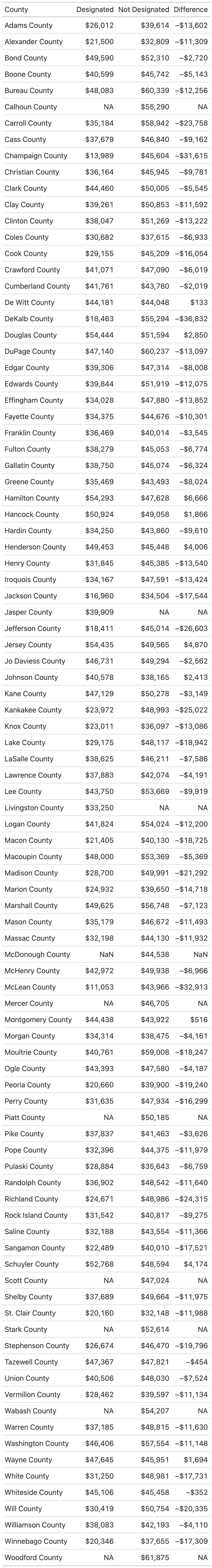
ozs |> 
  filter(state == "Illinois") |> 
  group_by(county, Designated) |> 
  summarise(
    Income = mean(medhhincome2014_tract, na.rm=TRUE)) |> pivot_wider(names_from = Designated, values_from = Income) |> 
  mutate(Difference = Designated - `Not Designated`) |> 
  ungroup() |> 
  gt() |> 
  fmt_currency(2:4, decimals = 0) |> 
  cols_label(county = "County")

County	Designated	Not Designated	Difference
Adams County	$26,012	$39,614	−$13,602
Alexander County	$21,500	$32,809	−$11,309
Bond County	$49,590	$52,310	−$2,720
Boone County	$40,599	$45,742	−$5,143
Bureau County	$48,083	$60,339	−$12,256
Calhoun County	NA	$55,290	NA
Carroll County	$35,184	$58,942	−$23,758
Cass County	$37,679	$46,840	−$9,162
Champaign County	$13,989	$45,604	−$31,615
Christian County	$36,164	$45,945	−$9,781
Clark County	$44,460	$50,005	−$5,545
Clay County	$39,261	$50,853	−$11,592
Clinton County	$38,047	$51,269	−$13,222
Coles County	$30,682	$37,615	−$6,933
Cook County	$29,155	$45,209	−$16,054
Crawford County	$41,071	$47,090	−$6,019
Cumberland County	$41,761	$43,780	−$2,019
De Witt County	$44,181	$44,048	$133
DeKalb County	$18,463	$55,294	−$36,832
Douglas County	$54,444	$51,594	$2,850
DuPage County	$47,140	$60,237	−$13,097
Edgar County	$39,306	$47,314	−$8,008
Edwards County	$39,844	$51,919	−$12,075
Effingham County	$34,028	$47,880	−$13,852
Fayette County	$34,375	$44,676	−$10,301
Franklin County	$36,469	$40,014	−$3,545
Fulton County	$38,279	$45,053	−$6,774
Gallatin County	$38,750	$45,074	−$6,324
Greene County	$35,469	$43,493	−$8,024
Hamilton County	$54,293	$47,628	$6,666
Hancock County	$50,924	$49,058	$1,866
Hardin County	$34,250	$43,860	−$9,610
Henderson County	$49,453	$45,448	$4,006
Henry County	$31,845	$45,385	−$13,540
Iroquois County	$34,167	$47,591	−$13,424
Jackson County	$16,960	$34,504	−$17,544
Jasper County	$39,909	NA	NA
Jefferson County	$18,411	$45,014	−$26,603
Jersey County	$54,435	$49,565	$4,870
Jo Daviess County	$46,731	$49,294	−$2,562
Johnson County	$40,578	$38,165	$2,413
Kane County	$47,129	$50,278	−$3,149
Kankakee County	$23,972	$48,993	−$25,022
Knox County	$23,011	$36,097	−$13,086
LaSalle County	$38,625	$46,211	−$7,586
Lake County	$29,175	$48,117	−$18,942
Lawrence County	$37,883	$42,074	−$4,191
Lee County	$43,750	$53,669	−$9,919
Livingston County	$33,250	NA	NA
Logan County	$41,824	$54,024	−$12,200
Macon County	$21,405	$40,130	−$18,725
Macoupin County	$48,000	$53,369	−$5,369
Madison County	$28,700	$49,991	−$21,292
Marion County	$24,932	$39,650	−$14,718
Marshall County	$49,625	$56,748	−$7,123
Mason County	$35,179	$46,672	−$11,493
Massac County	$32,198	$44,130	−$11,932
McDonough County	NaN	$44,538	NaN
McHenry County	$42,972	$49,938	−$6,966
McLean County	$11,053	$43,966	−$32,913
Mercer County	NA	$46,705	NA
Montgomery County	$44,438	$43,922	$516
Morgan County	$34,314	$38,475	−$4,161
Moultrie County	$40,761	$59,008	−$18,247
Ogle County	$43,393	$47,580	−$4,187
Peoria County	$20,660	$39,900	−$19,240
Perry County	$31,635	$47,934	−$16,299
Piatt County	NA	$50,185	NA
Pike County	$37,837	$41,463	−$3,626
Pope County	$32,396	$44,375	−$11,979
Pulaski County	$28,884	$35,643	−$6,759
Randolph County	$36,902	$48,542	−$11,640
Richland County	$24,671	$48,986	−$24,315
Rock Island County	$31,542	$40,817	−$9,275
Saline County	$32,188	$43,554	−$11,366
Sangamon County	$22,489	$40,010	−$17,521
Schuyler County	$52,768	$48,594	$4,174
Scott County	NA	$47,024	NA
Shelby County	$37,689	$49,664	−$11,975
St. Clair County	$20,160	$32,148	−$11,988
Stark County	NA	$52,614	NA
Stephenson County	$26,674	$46,470	−$19,796
Tazewell County	$47,367	$47,821	−$454
Union County	$40,506	$48,030	−$7,524
Vermilion County	$28,462	$39,597	−$11,134
Wabash County	NA	$54,207	NA
Warren County	$37,185	$48,815	−$11,630
Washington County	$46,406	$57,554	−$11,148
Wayne County	$47,645	$45,951	$1,694
White County	$31,250	$48,981	−$17,731
Whiteside County	$45,106	$45,458	−$352
Will County	$30,419	$50,754	−$20,335
Williamson County	$38,083	$42,193	−$4,110
Winnebago County	$20,346	$37,655	−$17,309
Woodford County	NA	$61,875	NA

Note that cols_label allows us to adjust column labels by supplying the variable name and then the desired name of the column.

gt provides a nice workflow example to show you step by step how you might apply formatting options to style a table. Also see the reference guide for specific formats.

Saving a Table

We can easily use code to insert a table into our document, but what if you want to save it out as a separate file? The gtsave() command allows you to save your formatted table in a variety of formats.

Code

ozs |> 
  filter(state == "Illinois") |> 
  group_by(county, Designated) |> 
  summarise(
    Income = mean(medhhincome2014_tract, na.rm=TRUE)) |> pivot_wider(names_from = Designated, values_from = Income) |> 
  mutate(Difference = Designated - `Not Designated`) |> 
  ungroup() |> 
  gt() |> 
  fmt_currency(2:4, decimals = 0) |> 
  cols_label(county = "County") |> 
  gtsave("il_difference.png", "/output")

And here’s the actual table that was produced:

Lab Evaluation

In evaluating your lab submission, we’ll be paying attention to the following:

As you get into the lab, please feel welcome to ask us questions, and please share where you’re struggling with us and with others in the class.