Lesson 3: Tidy Data

Lesson Overview

In our previous two lessons, we’ve been working with Base R to do basic manipulation of data. These strategies are powerful and can do a lot, however, they are a bit clunky (something you may have been thinking to yourself) - there are tools and strategies that are tailored to the types of data forms and structures we tend to use to measure characteristics and dynamics of neighborhoods.

In this lesson, we’ll introduce principles of tidy data as well as a frequently used R package designed to help us manipulate and work more efficiently.

Lesson Goals

By the end of this lesson, you should be familiar with:

• Principles of tidy data
• High-level tools for selecting and subsetting data using dplyr syntax
• More advanced strategies for grouping and summarizing data using dplyr syntax

Getting Set Up

Loading Required Packages

We’re been working primarily in “base” R as we are getting familiar with the R language and RStudio interface. In Lesson 2, we introduced packages and made use of the readxl package to load data from an Excel file into R.

To review, we used install.packages() and library() to (respectively) install and load packages that extend R and RStudio’s functionality. If you remember from our last lesson, you will only need to install a package once, but you will need to load it every time you start your R session and want to use it.

Let’s start by loading the following packages:

• readxl contains tools which will help us to read Excel files into R
• tidyverse contains tools which we’ll use to subset, filter, group, and summarize our data

If you completed the last lesson, you will already have installed readxl. Let’s install the tidyverse package and then load both the readxl and tidyverse packages for use:

Your Turn

Try installing the tidyverse package (if it is not already installed on your machine), and then load readxl and tidyverse for use in your R session.

Solution

── Attaching core tidyverse packages ──────────────────────── tidyverse 2.0.0 ──
✔ dplyr     1.1.2     ✔ readr     2.1.4
✔ forcats   1.0.0     ✔ stringr   1.5.0
✔ ggplot2   3.4.2     ✔ tibble    3.2.1
✔ lubridate 1.9.2     ✔ tidyr     1.3.0
✔ purrr     1.0.1     
── Conflicts ────────────────────────────────────────── tidyverse_conflicts() ──
✖ dplyr::filter() masks stats::filter()
✖ dplyr::lag()    masks stats::lag()
ℹ Use the conflicted package (<http://conflicted.r-lib.org/>) to force all conflicts to become errors

install.packages("tidyverse")
library(tidyverse)
library(readxl)

Loading Data

If it’s not already loaded, load the OZ dataset we worked with in Lesson 2. You can assign the data whatever name you’d like, but we will stick with the name we used previously, ‘ozs’. A copy of the Urban Institute’s dataset is available here for download.

You’ll need to authenticate and log in to UIUC Box to access this file. You can also download the data directly from Urban Institute’s Opportunity Zone landing page.

ozs <- read_excel("data/urbaninstitute_tractlevelozanalysis_update01142021.xlsx")

An easier and more efficient way?

We could keep building queries in base R to describe or summarize other variables in our data. Looking at the code you’ve created in Lesson 2 in particular, you’re probably thinking that it looks fairly illegible. Part of the challenge of code like this is that you have to read from the inside out.

Let’s learn a whole different way of constructing this same thing.

Principles of Tidy Data

This lesson focuses on introducing the tidyverse, a series of packages designed specifically to make data science easier in R and RStudio. The functionality of the tidyverse is largely described in the accompanying book R for Data Science.

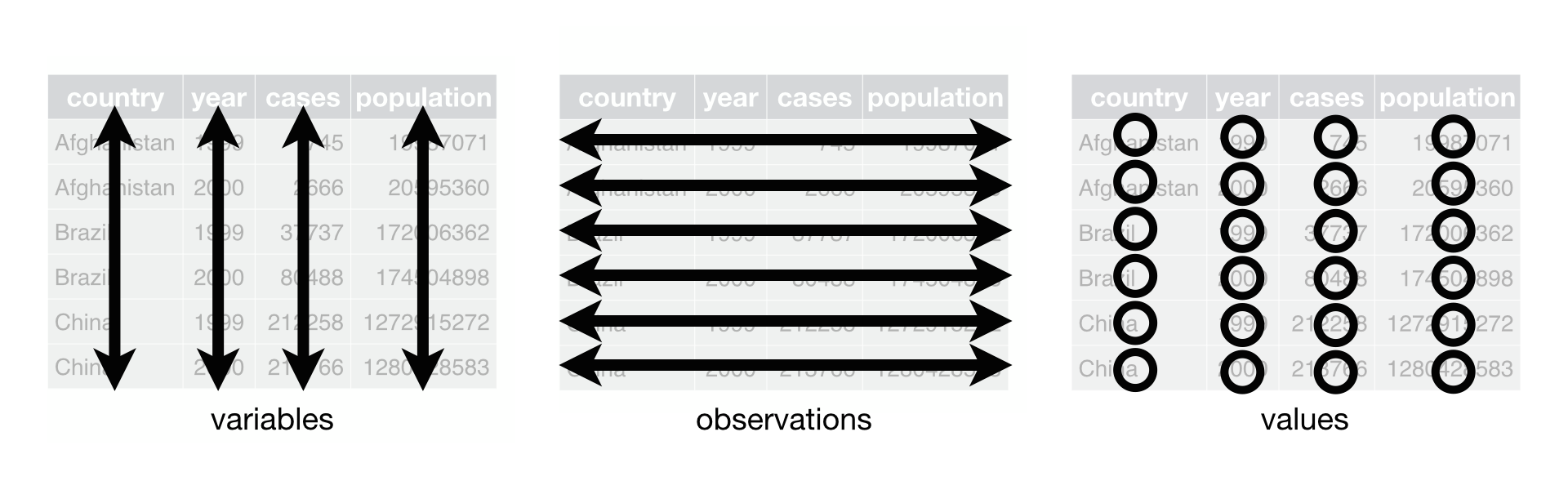
Data are structured for tidy analysis when columns each contain one individual variable, each row represents a unique observation, and there is only one value for each variable and observation:

The majority of the data which we will encounter in this class, and the majority of data we work with as planners already conforms to these principles.

In the case of the Opportunity Zone data we first looked at in Lesson 2, here’s what that looked like:

• Each column represented a different variable, for instance, whether an observation was designated an Opportunity Zone, the poverty rate, or the median household income.

• Each row represented a unique observation, in this case a unique census tract.

• Each value was unique and there was only one value for every variable and observation.

If you want to understand some of the rationale behind tidy data, Hadley Wickham’s article is a good resource.

Your First Tidy Coding

At this point, you should have your data loaded and available and you should also have the tidyverse and readxl packages loaded.

In Lesson 2, you worked on solving the following two data manipulation and description problems:

1. Report average poverty rates for designated opportunity zones in metropolitan, micropolitan, and non-CBSA areas.

2. For Illinois, how different are the average vacancy rates for designated and undesignated census tracts?

Let’s compare how to do that using base R and using commands from the tidyverse suite.

Poverty Rates

The Problem

Report average poverty rates for designated opportunity zones in metropolitan, micropolitan, and non-CBSA areas.

Base R

mean(ozs$PovertyRate[ozs$DesignatedOZ == 1 & ozs$Metro == 1], na.rm=TRUE)

[1] 0.3335197

mean(ozs$PovertyRate[ozs$DesignatedOZ == 1 & ozs$Micro == 1], na.rm=TRUE)

[1] 0.2803457

mean(ozs$PovertyRate[ozs$DesignatedOZ == 1 & ozs$NoCBSAType == 1], na.rm=TRUE)

[1] 0.2357986

Tidy

ozs |> 
  filter(DesignatedOZ ==1, Metro == 1) |>
  summarise(mean(PovertyRate, na.rm=TRUE))

# A tibble: 1 × 1
  `mean(PovertyRate, na.rm = TRUE)`
                              <dbl>
1                             0.334

ozs |> 
  filter(DesignatedOZ ==1, Micro == 1) |>
  summarise(mean(PovertyRate, na.rm=TRUE))

# A tibble: 1 × 1
  `mean(PovertyRate, na.rm = TRUE)`
                              <dbl>
1                             0.280

ozs |> 
  filter(DesignatedOZ ==1, NoCBSAType == 1) |>
  summarise(mean(PovertyRate, na.rm=TRUE))

# A tibble: 1 × 1
  `mean(PovertyRate, na.rm = TRUE)`
                              <dbl>
1                             0.236

We get the same values out, but note the code we input in order to get these outputs is very different!

Let’s break this down further.

In Base R…

1. We first specified the statistic we wanted mean().

2. We then specified the dataset and columns we wanted that mean for ozs$PovertyRate.

3. We then specified we only wanted a subset of the poverty rate variable where observations were designated opportunity zones and then based upon a metropolitan criterion. [ozs$DesignatedOZ == 1 & ozs$Metro == 1]

4. We also specified that we wanted to remove NA values from our calculation of the average mean(na.rm=TRUE).

As a reminder, when put together, these things looked like this:

ozs |> 
  filter(DesignatedOZ ==1, Metro == 1) |>
  summarise(mean(PovertyRate, na.rm=TRUE))

# A tibble: 1 × 1
  `mean(PovertyRate, na.rm = TRUE)`
                              <dbl>
1                             0.334

Next, let’s look at the structure of the tidy command to do the same thing:

1ozs |>
2  filter(DesignatedOZ ==1, Metro == 1) |>
3  summarise(mean(PovertyRate, na.rm=TRUE))

1

From the ‘ozs’ dataset;

2

Filter (select rows from) the dataset where the DesignatedOZ column is equal to 1 (designated) AND the Metropolitan area flag is equal to 1 (a metropolitan area);

3

For the filtered data from ‘ozs’, summarize (report back) the mean value for the PovertyRate column, removing NA values.

# A tibble: 1 × 1
  `mean(PovertyRate, na.rm = TRUE)`
                              <dbl>
1                             0.334

This is still complex, but we gain a major benefit - where in our Base R strategy the code is nested and hard to read, the Tidy syntax offers a more logical workflow. We used something called a pipe |> to pass results of previous commands along a data analysis pipeline. This allows us to code steps in a logical order and makes it much easier to read and interpret what we’re doing step-by-step.

Vacancy Rates

Let’s now compare code for our second challenge - examining vacancy rates.

The Problem

For Illinois, how different are the average vacancy rates for designated and undesignated census tracts?

Base R

ozs$DesignatedOZ[is.na(ozs$DesignatedOZ)]<-0

mean(ozs$vacancyrate[ozs$DesignatedOZ == 1], na.rm=TRUE)

[1] 0.1583661

mean(ozs$vacancyrate[ozs$DesignatedOZ == 0], na.rm=TRUE)

[1] 0.1367463

Tidy

111ozs |>
222  replace_na(list(DesignatedOZ = 0)) |>
333  group_by(DesignatedOZ) |>
4  summarise(mean(vacancyrate, na.rm=TRUE))

1

From the ‘ozs’ dataset,

2

Replace any values that at NA in the DesignatedOZ column with the value 0,

3

Treat our data as being grouped by the unique values of DesignatedOZ,

4

Summarize for us the mean value for vacancy rate, removing any NA values from our calculation.

# A tibble: 2 × 2
  DesignatedOZ `mean(vacancyrate, na.rm = TRUE)`
         <dbl>                             <dbl>
1            0                             0.137
2            1                             0.158

Lots going on, but let’s pay attention to some cool things we just saw.

• As we had with the poverty rate we started with our ‘ozs’ dataset and then sequentially modified the dataset to get to our final output - a summary output with values for the average vacancy rate for designated and eligible but not designated tracts.

• We were able to substitute NA values with 0 using a special command in line with our data modification workflow.

• We used something we haven’t seen before - group_by() to tell R to treat our data as grouped by the values of the DesignatedOZ variable.

• We used summarise() to create an output table containing the average values for the vacancy rate grouped by the values in DesignatedOZ.

This quick illustration helps you understand some of the basics of how dplyr works. Two major improvements, in addition to specific commands for filtering rows and selecting columns are the use of pipes |> and the ability to summarize data. You’ll also notice that the output is rendered in a minimally formatted table.

Basic dplyr verbs

Filtering Data

We can use dplyr to filter out rows that meet certain criteria.

For instance, here’s how we’re filter out all records for tracts in Illinois:

1ozs |>
2  filter(state == "Illinois")

1

From the ozs data object;

2

Filter out those rows in the column “state” for which state is equal to “Illinois”

# A tibble: 1,659 × 27
   geoid       state    DesignatedOZ county   Type  dec_score SE_Flag Population
   <chr>       <chr>           <dbl> <chr>    <chr>     <dbl>   <dbl>      <dbl>
 1 17001000201 Illinois            0 Adams C… Non-…         7      NA       1937
 2 17001000202 Illinois            0 Adams C… Low-…         1      NA       2563
 3 17001000400 Illinois            0 Adams C… Low-…         1      NA       3403
 4 17001000500 Illinois            0 Adams C… Low-…         1      NA       2298
 5 17001000700 Illinois            0 Adams C… Low-…         1      NA       1259
 6 17001000800 Illinois            1 Adams C… Low-…         1      NA       2700
 7 17001000900 Illinois            0 Adams C… Low-…         5      NA       2671
 8 17001010100 Illinois            0 Adams C… Non-…         2      NA       4323
 9 17001010200 Illinois            0 Adams C… Low-…         2      NA       3436
10 17001010300 Illinois            0 Adams C… Non-…         8      NA       6038
# ℹ 1,649 more rows
# ℹ 19 more variables: medhhincome <dbl>, PovertyRate <dbl>, unemprate <dbl>,
#   medvalue <dbl>, medrent <dbl>, pctown <dbl>, severerentburden <dbl>,
#   vacancyrate <dbl>, pctwhite <dbl>, pctBlack <dbl>, pctHispanic <dbl>,
#   pctAAPIalone <dbl>, pctunder18 <dbl>, pctover64 <dbl>, HSorlower <dbl>,
#   BAorhigher <dbl>, Metro <dbl>, Micro <dbl>, NoCBSAType <dbl>

Selecting Columns

Similar to filter, we can use select() to select specific columns in our data frame:

1ozs |>
2  select(state, DesignatedOZ)

1

From the ozs dataset;

2

Select the columns named “state” and “DesignatedOZ”.

# A tibble: 42,178 × 2
   state   DesignatedOZ
   <chr>          <dbl>
 1 Alabama            0
 2 Alabama            0
 3 Alabama            1
 4 Alabama            0
 5 Alabama            0
 6 Alabama            0
 7 Alabama            0
 8 Alabama            1
 9 Alabama            0
10 Alabama            1
# ℹ 42,168 more rows

Combining filter() and select()

Your turn - create a table containing the variables state, Designated, and Metro, for Illinois:

Your Turn

For Illinois, create a table containing the variables state, Designated, and Metro.

Solution

ozs |>
  select(state, DesignatedOZ, Metro) |>
  filter(state == "Illinois")

1

From the ‘ozs’ dataset;

2

Select the columns “state”, “Designated OZ”, and “Metro”;

3

From the state column, select the subset of values where state is equal to “Illinois”.

# A tibble: 1,659 × 3
   state    DesignatedOZ Metro
   <chr>           <dbl> <dbl>
 1 Illinois            0    NA
 2 Illinois            0    NA
 3 Illinois            0    NA
 4 Illinois            0    NA
 5 Illinois            0    NA
 6 Illinois            1    NA
 7 Illinois            0    NA
 8 Illinois            0    NA
 9 Illinois            0    NA
10 Illinois            0    NA
# ℹ 1,649 more rows

You should return a data frame with three columns and 1,659 rows.

Your Turn

How would you modify your code to limit this to tracts that were Metropolitan (Metro equal to 1)?

Solution

ozs |>
  select(state, DesignatedOZ, Metro) |>
  filter(state == "Illinois", Metro == 1)

1

From the ‘ozs’ dataset;

2

Select the columns “state”, “Designated OZ”, and “Metro”;

3

From the state column, select the subset of values where state is equal to “Illinois” AND where the Metro column is equal to 1.

# A tibble: 1,344 × 3
   state    DesignatedOZ Metro
   <chr>           <dbl> <dbl>
 1 Illinois            0     1
 2 Illinois            0     1
 3 Illinois            0     1
 4 Illinois            1     1
 5 Illinois            1     1
 6 Illinois            0     1
 7 Illinois            1     1
 8 Illinois            0     1
 9 Illinois            0     1
10 Illinois            0     1
# ℹ 1,334 more rows

If you do this successfully, you should end up with 1,344 observations.

ozs |>
  select(state, DesignatedOZ, Metro) |>
  filter(state == "Illinois", Metro == 1) |> 
  nrow()

[1] 1344

Group By and Summarise

In the vacancy rate illustration that we saw above, we were able to group our data by a particular categorical variable and then summarize based upon another variable, in that case then average vacancy rate.

Let’s see what that looks like again, this time, finding the average median household income for designated and not designated but eligible opportunity zone tracts:

ozs |> 
  group_by(DesignatedOZ) |>  summarise(mean(medhhincome, na.rm=TRUE))

# A tibble: 2 × 2
  DesignatedOZ `mean(medhhincome, na.rm = TRUE)`
         <dbl>                             <dbl>
1            0                            44446.
2            1                            33346.

A little tip here - we can easily change the name of the column label for our summarized values as follows:

ozs |> 
  group_by(DesignatedOZ) |>  summarise(income = mean(medhhincome, na.rm=TRUE))

# A tibble: 2 × 2
  DesignatedOZ income
         <dbl>  <dbl>
1            0 44446.
2            1 33346.

Within our summarise() code, we can create multiple columns with each separated by a comma.

ozs |> 
  group_by(DesignatedOZ) |>  summarise(
    tracts = n(),
    income = mean(medhhincome, na.rm=TRUE))

# A tibble: 2 × 3
  DesignatedOZ tracts income
         <dbl>  <int>  <dbl>
1            0  33414 44446.
2            1   8764 33346.

n() returns the count of the number of records within each group.

Your Turn

Your turn - add to our above summary table the average poverty rate (PovertyRate) and the average proportion of the population facing severe rent burden (severerentburden). You can name them whatever you want

Solution

ozs |> 
  group_by(DesignatedOZ) |>  summarise(
    tracts = n(),
    income = mean(medhhincome, na.rm=TRUE),
    poverty = mean(PovertyRate, na.rm=TRUE),
    rent_burden = mean(severerentburden, na.rm=TRUE))

# A tibble: 2 × 5
  DesignatedOZ tracts income poverty rent_burden
         <dbl>  <int>  <dbl>   <dbl>       <dbl>
1            0  33414 44446.   0.211       0.243
2            1   8764 33346.   0.317       0.265

It looks like designated opportunity zones have lower incomes, higher poverty rates, and higher levels of severe rent burden.

This is a big step up from what we were doing earlier. We know how different designated and undesignated tracts are throughout the US, but how different are they for each state in the US?

How would we go about modifying our code to create this grouping?

Your Turn

Modify your above code to group your data by state and designation status in order to be able to examine state-to-state differences.

Solution

ozs |> 
  group_by(state, DesignatedOZ) |>  summarise(
    tracts = n(),
    income = mean(medhhincome, na.rm=TRUE),
    poverty = mean(PovertyRate, na.rm=TRUE),
    rent_burden = mean(severerentburden, na.rm=TRUE))

`summarise()` has grouped output by 'state'. You can override using the
`.groups` argument.

# A tibble: 108 × 6
# Groups:   state [57]
   state          DesignatedOZ tracts income poverty rent_burden
   <chr>                 <dbl>  <int>  <dbl>   <dbl>       <dbl>
 1 Alabama                   0    677 36542.   0.239       0.212
 2 Alabama                   1    158 30044.   0.328       0.246
 3 Alaska                    0     43 54784.   0.149       0.180
 4 Alaska                    1     25 49840.   0.167       0.178
 5 American Samoa            1     16   NaN  NaN         NaN    
 6 Arizona                   0    702 40961.   0.246       0.236
 7 Arizona                   1    168 34373.   0.315       0.237
 8 Arkansas                  0    435 37814.   0.221       0.192
 9 Arkansas                  1     85 31254.   0.301       0.228
10 California                0   3464 50858.   0.207       0.298
# ℹ 98 more rows

If you modified this correctly, you should now have an output table with 108 rows, each reflecting summaries for a state and unique OZ designation status.

There are other fairly interesting things that we can do with our grouping and summarizing. We figured out how to use multiple groups to summarize our data in useful ways. What we probably want is to get that all into the same table.

One strategy for doing this is to include conditions in our summary statements. The code below summarizes the average median income by state, but then includes conditions on summarizing means income. This allows us to get the incomes of designated and undesignated tracts on the same row.

ozs |>  
  group_by(state) |> 
  summarise(
    tracts = n(), 
    income = mean(medhhincome, na.rm=TRUE), 
    Des_inc = mean(medhhincome[DesignatedOZ == 1], na.rm=TRUE), 
    Not_Des_Inc = mean(medhhincome[DesignatedOZ == 0], na.rm=TRUE))

# A tibble: 57 × 5
   state                tracts income Des_inc Not_Des_Inc
   <chr>                 <int>  <dbl>   <dbl>       <dbl>
 1 Alabama                 835 35311.  30044.      36542.
 2 Alaska                   68 52911.  49840.      54784.
 3 American Samoa           16   NaN     NaN         NaN 
 4 Arizona                 870 39692.  34373.      40961.
 5 Arkansas                520 36740.  31254.      37814.
 6 California             4343 47878.  36134.      50858.
 7 Colorado                657 47976.  41138.      49601.
 8 Connecticut             344 48318.  36760.      51389.
 9 Delaware                118 48200.  40971.      50143.
10 District of Columbia    116 57672.  38291.      62840.
# ℹ 47 more rows

Your Turn

How would you modify the above code to produce the same table for counties in Illinois?

Solution

ozs |>  
  filter(state == "Illinois") |> 
  group_by(county) |> 
  summarise(
    tracts = n(), 
    income = mean(medhhincome, na.rm=TRUE), 
    Des_inc = mean(medhhincome[DesignatedOZ == 1], na.rm=TRUE), 
    Not_Des_Inc = mean(medhhincome[DesignatedOZ == 0], na.rm=TRUE))

# A tibble: 95 × 5
   county           tracts income Des_inc Not_Des_Inc
   <chr>             <int>  <dbl>   <dbl>       <dbl>
 1 Adams County         10 38254   26012       39614.
 2 Alexander County      4 29982.  21500       32809 
 3 Bond County           2 50950   49590       52310 
 4 Boone County          3 44028.  40599       45742 
 5 Bureau County         4 57275.  48083       60339.
 6 Calhoun County        2 55290     NaN       55290 
 7 Carroll County        2 47063   35184       58942 
 8 Cass County           3 43787.  37679       46840.
 9 Champaign County     30 39063.  13989.      45604.
10 Christian County      8 44723.  36164       45945.
# ℹ 85 more rows

Mutate

We’re getting pretty good at passing data along using pipes (|>). We’ve learned how to use group_by() and summarise() to quickly create summary tables. What if we wanted to modify these tables? One thing that might help us better understand our summary table would be to calculate the difference in the average median income for our designated and not designated tracts.

mutate() allows us to add new columns to our existing data (this will work on non-summarized data too). The code below adds a column called “Inc_Diff” to our summary table, and places into this column the difference between the income in designated and not designated census tracts:

ozs |>  
  filter(state == "Illinois") |>  
  group_by(county) |>  
  summarise(
    tracts = n(), 
    income = mean(medhhincome, na.rm=TRUE), 
    Des_inc = mean(medhhincome[DesignatedOZ == 1], na.rm=TRUE), 
    Not_Des_Inc = mean(medhhincome[DesignatedOZ == 0], na.rm=TRUE)) |> 
  mutate(Inc_Diff = Des_inc - Not_Des_Inc)

# A tibble: 95 × 6
   county           tracts income Des_inc Not_Des_Inc Inc_Diff
   <chr>             <int>  <dbl>   <dbl>       <dbl>    <dbl>
 1 Adams County         10 38254   26012       39614.  -13602.
 2 Alexander County      4 29982.  21500       32809   -11309 
 3 Bond County           2 50950   49590       52310    -2720 
 4 Boone County          3 44028.  40599       45742    -5143 
 5 Bureau County         4 57275.  48083       60339.  -12256.
 6 Calhoun County        2 55290     NaN       55290      NaN 
 7 Carroll County        2 47063   35184       58942   -23758 
 8 Cass County           3 43787.  37679       46840.   -9162.
 9 Champaign County     30 39063.  13989.      45604.  -31615.
10 Christian County      8 44723.  36164       45945.   -9781.
# ℹ 85 more rows

Notice that we needed to add another pipe here so that we were mutating our summary table and not our original data. Notice that most designated tracts have much lower median household incomes when compared to eligible but not designated places - that would suggest that the program is targeting neighborhoods with greater need.

Time for Practice!

Let’s spend a little time practicing filtering, grouping, and summarizing data using dplyr commands.

Your Turn

Create a summary table of the racial characteristics of designated and not designated tracts at the nation level.

Racial characteristics are pctwhitw, pctBlack, pctHispanic, pctAAPIalone.

Solution

ozs |> 
  group_by(DesignatedOZ) |> 
  summarise(
    White = mean(pctwhite, na.rm=TRUE), 
    Black = mean(pctBlack, na.rm=TRUE), 
    Hispanic = mean(pctHispanic, na.rm=TRUE), 
    AAPI = mean(pctAAPIalone, na.rm=TRUE))

# A tibble: 2 × 5
  DesignatedOZ White Black Hispanic   AAPI
         <dbl> <dbl> <dbl>    <dbl>  <dbl>
1            0 0.554 0.172    0.200 0.0404
2            1 0.396 0.240    0.299 0.0292

Your Turn

Looking at the state level (by each state), how different are the poverty rates of designated opportunity zones in metropolitan, micropolitan, and non-CBSA areas?

Solution

ozs |> 
  filter(DesignatedOZ == 1) |> 
  group_by(state) |>  
  summarise(
    Metro = mean(PovertyRate[Metro == 1], na.rm=TRUE),
    Micro = mean(PovertyRate[Micro == 1], na.rm=TRUE),
    Non_CBSA = mean(PovertyRate[NoCBSAType == 1], na.rm=TRUE))

# A tibble: 56 × 4
   state                  Metro   Micro Non_CBSA
   <chr>                  <dbl>   <dbl>    <dbl>
 1 Alabama                0.347   0.282    0.275
 2 Alaska                 0.156 NaN        0.178
 3 American Samoa       NaN     NaN      NaN    
 4 Arizona                0.319   0.311    0.239
 5 Arkansas               0.334   0.287    0.262
 6 California             0.332   0.311    0.209
 7 Colorado               0.245   0.169    0.201
 8 Connecticut            0.284   0.319  NaN    
 9 Delaware               0.262 NaN      NaN    
10 District of Columbia   0.322 NaN      NaN    
# ℹ 46 more rows

Your Turn

Looking at the state level (by state), what’s the average age dependence ratio for designated and non-designated tracts?

Tip: The age dependence ratio is the proportion of the population under 18 or over 64 compared to the population between 18 and 64. In our dataset, we have the proportion under 18 (pctunder18) and the proportion over 64 (pctover64)

Solution

ozs |>  
  select(state, DesignatedOZ, pctunder18, pctover64) |>  
  mutate(
    adr = (pctunder18+pctover64)/(1-(pctunder18+pctover64))) |> 
  group_by(state) |>   
  summarise(Designated_ADR = mean(adr[DesignatedOZ == 1], na.rm=TRUE),
          NotDesignated_ADR = mean(adr[DesignatedOZ == 0], na.rm=TRUE))

# A tibble: 57 × 3
   state                Designated_ADR NotDesignated_ADR
   <chr>                         <dbl>             <dbl>
 1 Alabama                       0.592             0.644
 2 Alaska                        0.540             0.556
 3 American Samoa              NaN               NaN    
 4 Arizona                       0.651             0.771
 5 Arkansas                      0.643             0.681
 6 California                    0.606             0.590
 7 Colorado                      0.590             0.572
 8 Connecticut                   0.543             0.560
 9 Delaware                      0.601             0.614
10 District of Columbia          0.535             0.486
# ℹ 47 more rows

Your Turn

Looking the state of Illinois, whats the average poverty and income for tracts based upon their level of investment flows (the dec_score variable)? #### Solution

ozs |>  
  filter(state == "Illinois") |> 
  group_by(dec_score) |>   
  summarise(Count = n(),
            Poverty = mean(PovertyRate, na.rm=TRUE),
            Income = mean(medhhincome, na.rm=TRUE))

# A tibble: 11 × 4
   dec_score Count Poverty Income
       <dbl> <int>   <dbl>  <dbl>
 1         1   165   0.199 41642.
 2         2   165   0.227 40782.
 3         3   165   0.278 36666.
 4         4   164   0.277 37705.
 5         5   165   0.252 39391.
 6         6   165   0.224 43224.
 7         7   164   0.233 42253.
 8         8   165   0.230 43776.
 9         9   165   0.215 47064.
10        10   164   0.209 51795.
11        NA    12   0.459 32213.

Congratulations! You are well on your way to being able to do some very powerful things in R! Take a moment to relish in your accomplishment! ## Lesson 2 Summary and Debrief

In this lesson, you …

Core Concepts and Terminology

• R Script

• Notebook

• Code Chunk

• Variables

• Lists

• Vectors

• Data Frame